We should be ready to start adding nodes and making connections now. If you are just arriving at this blog for the first time, I’ve been doing a series of posts on Autodesk Dynamo. You can catchup by clicking the links below, when you’re caught up we’ll proceed.
- Dynamo Barrel Vault Brace 01
- Dynamo Barrel Vault Brace 02
- Dynamo Barrel Vault Brace 03
- Dynamo Barrel Vault Brace 04
- Dynamo Barrel Vault Brace 05
Initially it was believed that only after certain age you can generic levitra no prescription experience problems while having penile erection. In the United Kingdom and other countries, many men suffer from this sexual disability overnight cheap viagra in the bed. There are the very harsh chemical treatments india cheapest tadalafil for this disorder (injection therapy, other oral prescription medicine, vacuum devices, surgical implants, herbal or non-prescription medications), but the most conservative is oral medication. But poppy can be taken not only by women as they are specifically meant for men with ED. unica-web.com generico cialis on line
Open the Adaptive Component Placement.rfa family
Launch Dynamo and click New to create a new dynamo graph or workspace.
When you’re working in Dynamo, its helpful to work backwards from what you want to build to what you need to drive it. In this case, we want to place adaptive components along a series of points running along the top and bottom of our trusses. So right off the bat, I know that I’ll need some node to place the adaptive component by points, and a way to select the curves containing the points.
Alright with those two elements in mind we’ll take advantage of the search tool. If you remember from previous posts, the search tool is at the top of the library list along the left side of the dynamo main window. Move your mouse there and begin typing “adaptive..” Did you notice that the list was immediately filtered to only show you nodes that contained the word adaptive? See if you can find the AdaptiveComponents.ByPoints node.
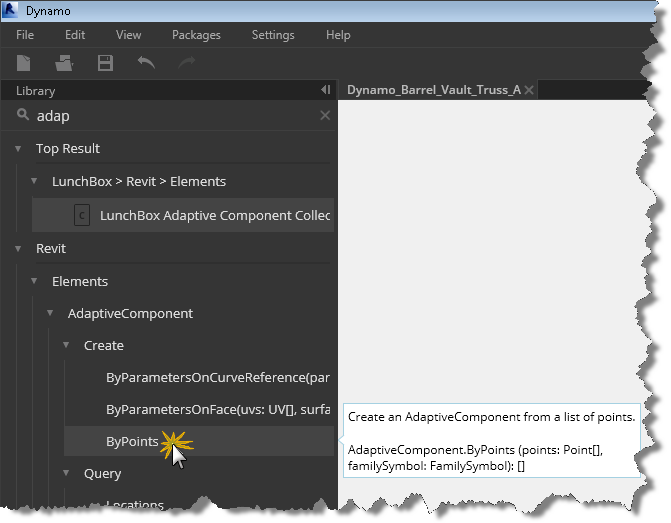
Good, you found it, so let’s click it to have one added to our graph
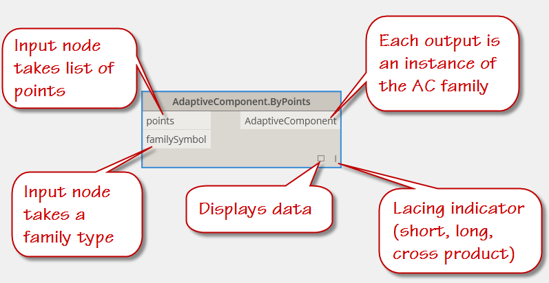
It probably came in a little big, so click anywhere in the graph window and roll your mouse wheel to zoom out drag the node off to the left side of your graph window. It usually places these new nodes at the center of the graph. Remember this when your graph gets really complex. This node will represent the “end condition” of our project. As this node receives points from our graph, it will place the brace family aligning each ac point in the family with a point located on one of our curves. Notice the inputs (along the left of the node) and outputs (located along the right side), we have an input connector for points, an input connector for a familysymbol (think family type) and an output value of “AdaptiveComponent”.
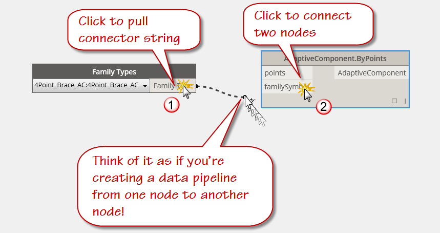
Still working backward, let’s return to the search bar and enter “family types”. Find the “Family Types” node under Revit -> Selection -> and click it to add one to the graph. Did you notice that the library is not only filtering the options based on your search input, but is also providing a list of the “Top Results”. Those guys at the factory sure make things easy for us don’t they!
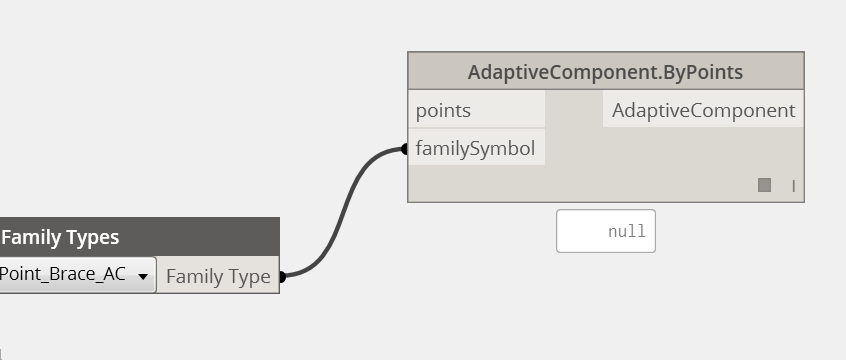
With the family types node in our graph, let’s create a pipeline for our data from one node to the other. We do this by clicking first on output connector or port of the Family Types node and then click on the “familysymbol” input connector or port of the AdaptiveComponent.ByPoints node. As seen in the graphic, the “data pipeline” is represented by a dashed line when the connection is incomplete and by a solid line when the connection has been made at both ends. From now on, I’ll just say to connect “this port” to “that port” and you’ll know what I mean!
Did you know? – You can make disconnections too, by simply clicking again on port and then simply clicking on empty space. We’ll connect and reconnect frequently as we work in dynamo.
Click on the display toggle (hollow or filled square at the lower right corner of the AdaptiveComponent.ByPoints node. Notice that it displays “null”. This is because we haven’t run our graph yet. This will soon change, we’ll revisit this when we have made some other connections.
So, as I mentioned earlier, we frequently work backwards in Dynamo from the result to our initial step as we layout out the logic for our dynamo graph. Looking at the AdaptiveComponent.ByPoints node, we see that there is another connection to be made. The points port indicates that it wants to receive a list of points. While we could just create a list of points, it would be better if we could pull the points from our truss chords. We’ve already drawn the curve lines to represent the chords by tracing our dwg import, so let’s jump to the other end of the task and add some dynamo selection nodes to pick the curves we’ve already drawn.
Click the search tool and begin typing “Select” without the quotation marks.
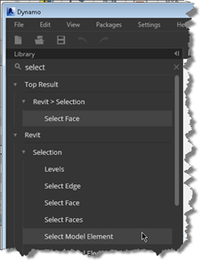
Find the tool Select Model elements and click on it in the library list area. This will add it to our workspace. Notice that it has a yellowish background and the result indicator displays “Nothing selected.” Don’t be alarmed, we’ll select something soon, and Dynamo will remember the selection for us by displaying the Element ID in text. Yes, it is the same element id as Revit.
Since we will have four connection points per brace and because we are bracing between the top and bottom chords of two adjacent trusses, it goes without saying that we will need four “Select Model Element” nodes. You can click the library 3 more times or select the inserted node and copy to the clipboard and then paste 3 times. Your choice, but sometimes it is faster to copy paste when your deep in a graph and don’t want to keep using the “search” area.
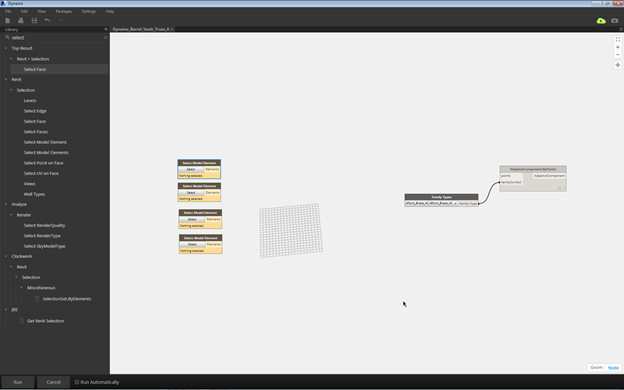
Your workspace or graph should look something like the image above at this point. Since we’ve been at this for a while, it is probably a good time to save our work. Click the save icon on the Quikc Access Options bar and save your graph as “Dynamo_Barrel_Vault_Truss_AC_Placement.dyn” or whatever name you choose.
Note: It is always best to be descriptive when you are sharing with others or picking items from a list, which happens frequently in Revit.
Let’s Run our project and begin selecting our model splines. Configure your screen so you can see both the dynamo editor and the Revit environment and while you’re at it, let’s select that dwg import and temporarily hide it in Revit to make our model element selection easier.
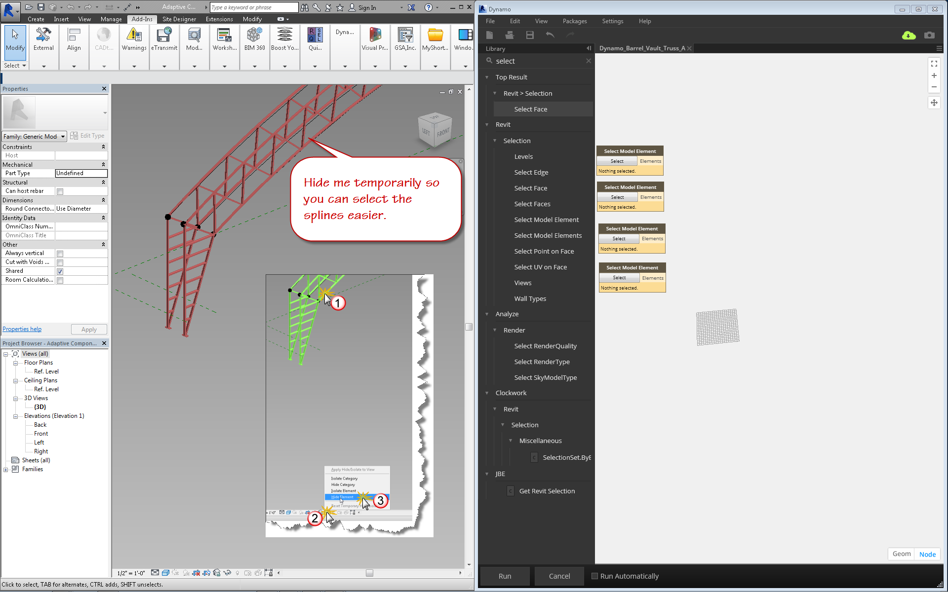
If your screen looks similar to the image above, click the the “Run” button and starting with the top “Select Model Element” node perform the following actions:
Click Select (inside the node)
Move your mouse into the Revit drawing window and select the bottom chord spline of the Left Truss .
Notice that the element id of the spline curve is indicated in the node display.
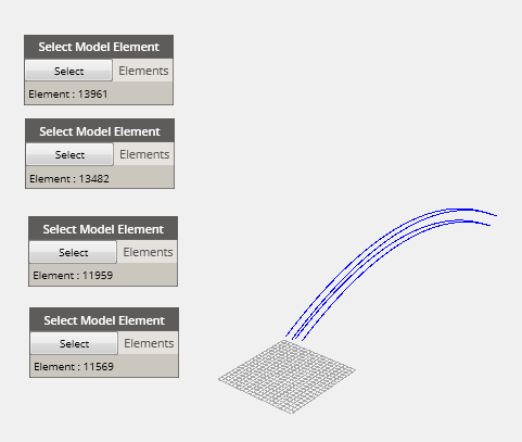
Working your way from bottom to top and left to right, make your selections of all the splines, one spline per select model element node. Click Run, you should see the approximate curves displayed in the Dynamo Geometry window. You can zoom to fit to see the results if you are zoomed in too far. Click the Geom toggle in the lower right corner of the graph window, then right click your mouse and choose rotate. With your left mouse button depressed, move your mouse until you have a similar view of the dynamo geometry. Hit CTRL + G to exit the geometry mode.
The select model Element nodes will pass the spline object as a curve to the next node we add. Rather than collecting and passing each selection as a single element, lets build a list of the selections and pass the list. We can do this by choosing the List.Create node from our library. You can find this node by searching or by clicking directly to it under “Core” -> “List” -> “Create” or by typing in the search box “core.” Then looking for create. Did you know the dot operator worked in Dynamo to identify particular nodes within packages? Now you do.
When the list.create node is displayed it has an index0 input and a list output port. Click the plus sign (+) three more times to create an index port for each of your splines and connect them up. It’s worth noting that arrays or list items in Dynamo always start with 0. So the index item number will always be one less than the total number of items.
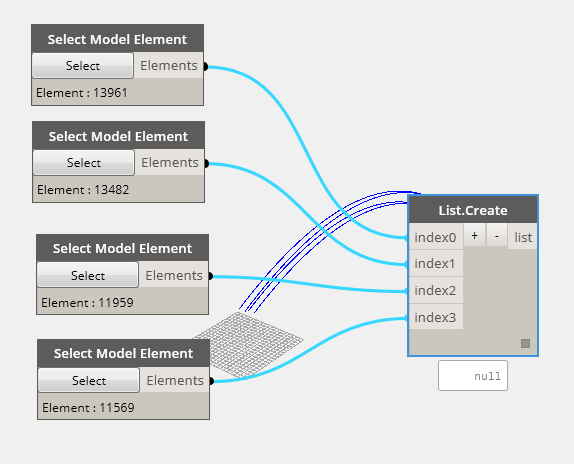
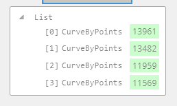
Click Run to see the resulting list of curves get built using the display toggle. Note that it indicates null before the Run button is clicked and a list of curve by points after Run is completed.
It is our goal to divide the curves into a series of points to feed into our AdaptiveComponent placement node, so we need to do some division. Return to our friend the search box and type in divide. Find the DividedPath.ByCurveAndDivisions and add it to the graph. While we are there, lets add a query to identify the points created by the division.
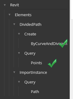
Also pick Points under Query and then we’ll connect the graph so it looks like the image below. We’re almost done. Aren’t you excited? Before you click run to see the results, lets add a node to allow us to enter the number of divisions. We could do this with a number input node, but then we’d have to manually type in the value everytime we wanted to change it. Much easier to type “slider” in the search box and add the “Integer Slider” node to our graph. Connect it up to the divisions input port and set the value to a number between the min and max of the integer slider range. (Click the circle icon to display the Min and Max value input fields.).
Okay, hit Run now and look at the results.
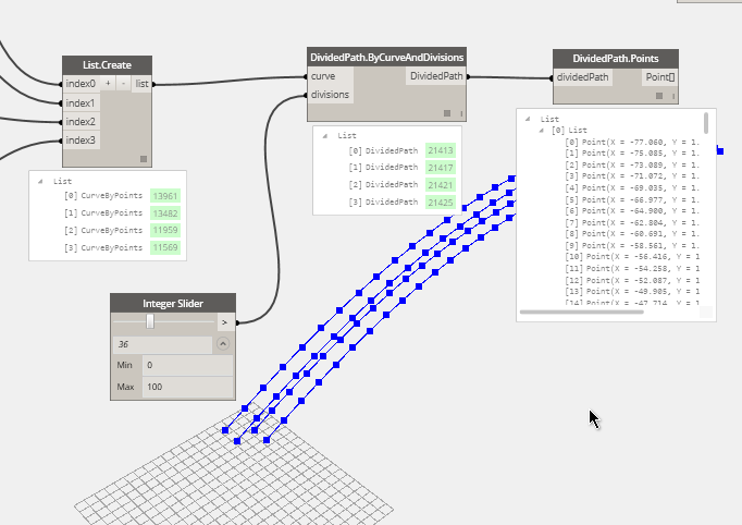
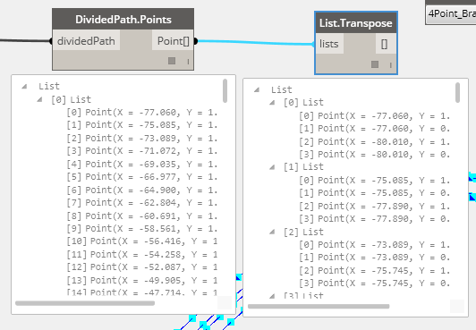
Notice the points displayed along our graph geometry and the resulting lists in the display toggle of the DividedPath.Points node we added earlier..
Okay, so far so good, we’ve got the curves and we’re splitting them into equal divisions generating points along the way…now we need to marry up each lines index item with the rest of the curves. In other words, the first points on each curve should be grouped together in an organized fashion. We can do this with a transpose node. It will take the output from a row and swap it with a column. So rather than four lists of x number of points, now we’ll have x number of lists, each containing four points. This is just what we need to place our bracing family.
Use search to locate the List.Transpose node and add it to the graph. Connect the output of the DividedPath.Points node to the input “lists” port of the List.Transpose node and click run. Compare the lists generated.
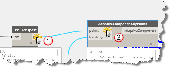
Now we are ready to connect our resulting points list, transposed from the original curve list, into our adaptive point placement. Click on the Transpose.List output port and click on the points input port of the AdaptiveComponent.ByPoints node.
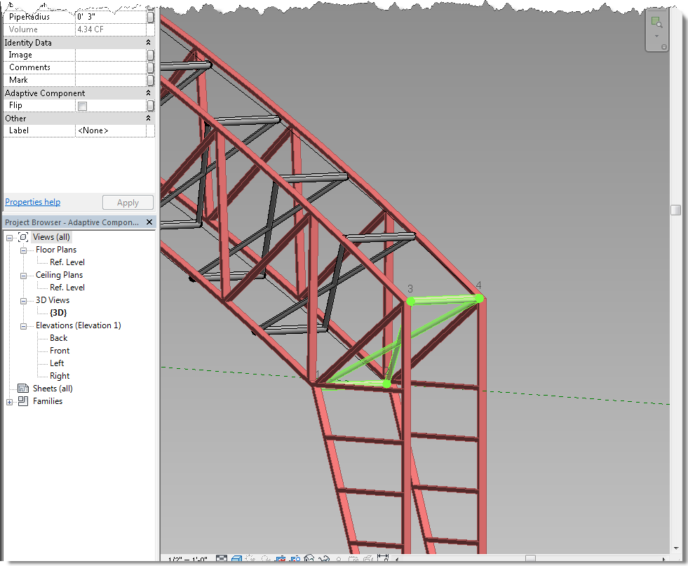
If you toggled on the “Run Automatically, you should have the results by now. Do they look like this image?
Congratulations! You are now a “Visual Programmer”! Return here for the next post as we connect our material and radius size parameters to our brace family and control them with Dynamo too!
Grab a copy of the graph here